고정 헤더 영역
상세 컨텐츠
본문
Introduction
So far in this course, we've learned about how neural networks can solve regression problems. Now we're going to apply neural networks to another common machine learning problem: classification. Most everything we've learned up until now still applies. The main difference is in the loss function we use and in what kind of outputs we want the final layer to produce.
여태까지는 신경망을 이용해서 회귀문제를 풀었다. 이번에는 또다른 대표적 머신러닝 문제인 분류문제를 풀어보자.
이제까지 배운 대부분의 것이 포함될 거다.
가장 큰 차이점은 손실함수와, 아웃풋을 내는 최종 레이어에서 뭘 내느냐다.
Binary Classification
Classification into one of two classes is a common machine learning problem. You might want to predict whether or not a customer is likely to make a purchase, whether or not a credit card transaction was fraudulent, whether deep space signals show evidence of a new planet, or a medical test evidence of a disease. These are all binary classification problems.
한 두개의 클래스로 분류하는 것은 머신 러닝 고유의 문제다. 고객이 들어왔을때 이 고객이 구매를 할 고객인지 아닌지도 알고 싶고 신용 카드 사용 내역 중에 부정 사용 내역을 가려내고 싶고 우주에서 날라오는 수많은 신호들 사이에서 외계 행성의 존재를 알리는 신호를 가려내고 싶고.... 이런 여러 종류의 문제가 분류 문제(classification)에 해당한다.
In your raw data, the classes might be represented by strings like "Yes" and "No", or "Dog" and "Cat". Before using this data we'll assign a class label: one class will be 0 and the other will be 1. Assigning numeric labels puts the data in a form a neural network can use.
만약 가지고 있는 데이터 셋에서 분류를 담당하는 클래스가 Yes, No, Dog, Cat과 같은 문자열로 구분되어 있다면 이 클래스들에 라벨링을 붙여줄 수 있다. 예를 들어 한 클래스가 0이면 다른 클래스를 1로 코딩하는 방법이다.
Accuracy and Cross-Entropy
정확도와 크로스 엔트로피
Accuracy is one of the many metrics in use for measuring success on a classification problem. Accuracy is the ratio of correct predictions to total predictions: accuracy = number_correct / total. A model that always predicted correctly would have an accuracy score of 1.0.
All else being equal, accuracy is a reasonable metric to use whenever the classes in the dataset occur with about the same frequency.
정확도(accuracy)는 모델의 분류 성능을 가늠하는 중요한 척도중 하나다. 정확도는 전체 예측에 대해서 맞는 예측 건에 대한 비율을 의미한다.
accuracy = number_correct / total_predict
만약 어떤 모델이 항상 정확한 분류를 해낸다면 이 모델의 정확도는 1.0이 된다.
(생략)
The problem with accuracy (and most other classification metrics) is that it can't be used as a loss function. SGD needs a loss function that changes smoothly, but accuracy, being a ratio of counts, changes in "jumps". So, we have to choose a substitute to act as the loss function. This substitute is the cross-entropy function.
이 정확도(accuracy)의 문제는 이 정확도라는 척도로는 로스 펑션(손실함수:Loss function)으로 사용할 수 없다는 점이다.
SGD로 사용되는 함수는 연속함수이고 완만한 변화가 있어야 하는데, accuracy는 말그대로 널뛴다.
따라서 우리는 모델에서 이 정확도를 대체할만한 손실함수를 모색해야 한다.
이 대체함수 중 하나가 cross-entropy (크로스 엔트로피; 교차 엔트로피) 함수다.
Now, recall that the loss function defines the objective of the network during training. With regression, our goal was to minimize the distance between the expected outcome and the predicted outcome. We chose MAE to measure this distance.
로스 펑션이 트레이닝 전 신경망의 오브젝트를 정의했던 것을 상기하자.
회귀문제에서 우리의 목표는 기대치와 예측치의 오차를 줄이는 것이었고 MAE를 통해 이 오차를 나타냈다.
For classification, what we want instead is a distance between probabilities, and this is what cross-entropy provides. Cross-entropy is a sort of measure for the distance from one probability distribution to another.
분류문제에서는 대신에 가능성/확률에 대한 거리가 필요하고 이것을 교차 엔트로피로 나타낸다.
교차 엔트로피란 하나의 확률분포에서 다른 확률 분포 사이의 거리를 나타내는 척도다.
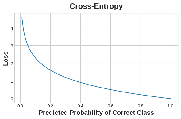
The idea is that we want our network to
predict the correct class with probability 1.0.
가장 이상적인 것은 해당 분류 모델이 가능성 1.0으로 정확한 모델을 분류해 내는 것이다.
The further away the predicted probability is from 1.0, the greater will be the cross-entropy loss.
예측된 확률이 1.0에서 멀어지면 멀어질 수록 크로스 엔트로피 손실은 점점 커진다.
The technical reasons we use cross-entropy are a bit subtle, but the main thing to take away from this section is just this: use cross-entropy for a classification loss; other metrics you might care about (like accuracy) will tend to improve along with it.
우리가 크로스 엔트로피를 사용하고 있는 이유를 설명하긴 어렵지만 여기서는 분류문제의 손실함수를 대체하기 위한 목적이라고 설명하고 있다.
(생략)
Making Probabilities with the Sigmoid Function
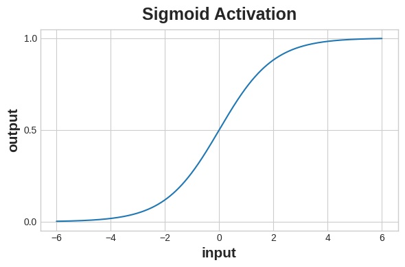
The cross-entropy and accuracy functions both require probabilities as inputs, meaning, numbers from 0 to 1. To covert the real-valued outputs produced by a dense layer into probabilities, we attach a new kind of activation function, the sigmoid activation.
크로스 엔트로피와 정확도 함수는 모두다 확률 값을 필요로 한다. 덴스 레이어가 만든 아웃풋을 확률로 변환하기 위해서는 새로운 종류의 활성화 함수를 고려해야 하는데, 여기서는 시그모이드 활성화 함수 (sigmoid activation function)를 소개한다.
.
To get the final class prediction, we define a threshold probability. Typically this will be 0.5, so that rounding will give us the correct class: below 0.5 means the class with label 0 and 0.5 or above means the class with label 1. A 0.5 threshold is what Keras uses by default with its accuracy metric.
최종적인 분류 예측을 얻기까지, 우리는 확률에 대한 경계값(threshold; 제한값; 임계값)을 정의해야 한다.
보통 0.5를 기주능로 한다.
예를 들어, 확률이 0.5 이하면 분류가 0이되고 0.5 이상이면 1이 되는 식이다.
Keras는 분류 문제에서 확률 경계값으로 0.5를 디폴트 값으로 하고 있다.
Example - Binary Classification
예시 - 바이너리 분류
Now let's try it out!
자 이제 해보자.
The Ionosphere dataset contains features obtained from radar signals focused on the ionosphere layer of the Earth's atmosphere. The task is to determine whether the signal shows the presence of some object, or just empty air.
The Ionosphere 데이터셋은 지구 대기에 있는 ionosphere (대기의 이온층은 뭘까?; 성층권의 전리층을 의미) 에서 수집되는 레이더 시그널과 관련된 피쳐 (feature; column; 특성명) 를 가진다.
이 모델의 목표는 위의 시그널을 분류해서 어떤 물체가 인식되는 시그널을 분류하는 것이다.
#데이터 셋 내용 생략
We'll define our model just like we did for the regression tasks, with one exception. In the final layer include a 'sigmoid' activation so that the model will produce class probabilities.
우리는 회구 모델에서 처럼 신경망 모델을 정의해 나가겠지만 첫 레이어는 시그모이드 활성화함수를 가진 레이어가 들어가고 이 모델에서 확률이 생성된다.
#파이썬 코드
from tensorflow import keras
from tensorflow.keras import layers
model = keras.Sequential([
layers.Dense(4, activation='relu', input_shape=[33]),
layers.Dense(4, activation='relu'),
layers.Dense(1, activation='sigmoid'),
])
#
Add the cross-entropy loss and accuracy metric to the model with its compile method. For two-class problems, be sure to use 'binary' versions. (Problems with more classes will be slightly different.) The Adam optimizer works great for classification too, so we'll stick with it.
여기에 크로스 엔트로피 로스와 정확도 척도를 넣는다.
#코드 아래
model.compile(
optimizer='adam',
loss='binary_crossentropy',
metrics=['binary_accuracy'],
)
#
The model in this particular problem can take quite a few epochs to complete training, so we'll include an early stopping callback for convenience.
이 모델은 트레이닝을 완료하는데 몇 에포크 정도면 충분할 것이다. 그래서 우리는 이른 시점에 callback 을 멈추도록 했다.
#파이썬코드
early_stopping = keras.callbacks.EarlyStopping(
patience=10,
min_delta=0.001,
restore_best_weights=True,
)
history = model.fit(
X_train, y_train,
validation_data=(X_valid, y_valid),
batch_size=512,
epochs=1000,
callbacks=[early_stopping],
verbose=0, # hide the output because we have so many epochs
)
#파이썬코드
We'll take a look at the learning curves as always, and also inspect the best values for the loss and accuracy we got on the validation set. (Remember that early stopping will restore the weights to those that got these values.)
이번에는 러닝 커브를 살펴보자. 로스 함수와 정확도 커브를 살펴보자.
#파이썬 코드
history_df = pd.DataFrame(history.history)
# Start the plot at epoch 5
history_df.loc[5:, ['loss', 'val_loss']].plot()
history_df.loc[5:, ['binary_accuracy', 'val_binary_accuracy']].plot()
print(("Best Validation Loss: {:0.4f}" +\
"\nBest Validation Accuracy: {:0.4f}")\
.format(history_df['val_loss'].min(),
history_df['val_binary_accuracy'].max()))
Best Validation Loss: 0.3534
Best Validation Accuracy: 0.8857
<실습계속>
'로봇-AI' 카테고리의 다른 글
| [딥러닝초급] Convnet + Relu (0) | 2025.02.26 |
|---|---|
| [딥러닝초급]the convolutional classifier (0) | 2025.02.24 |
| [딥러닝초급] Drop out and Batch Normalization (0) | 2025.02.18 |
| [딥러닝초급] Overfitting and Underfitting (0) | 2025.02.10 |
| [딥러닝기초] Stochastic Gradient Descent (0) | 2025.02.05 |


